Intro
Death rolling is a player made mini-game within World of Warcraft where two players alternate rolling a die between \([1-\text{previous players roll}]\) (the bounds are inclusive) until one player rolls a \(1\). The following is an example of a game:
Bob and Alice agree to death roll for 100 gold
Bob agrees to go first
Bob rolls 42 [1-100]
Alice rolls 12 [1-42]
Bob rolls 3 [1-12]
Alice rolls 1 [1-3]
Alice transfers 100 gold to Bob.
Now, as a player trying to maximize your returns should you go first or second? Bet large or small? Naturally, I wanted to find out.
Game
Death roll against a computer, alternating who goes first. Skip ahead to find out how to size your rolls. Keep in mind you can only roll whole integer amounts.
Simulation
My initial assumption was for very small bets the second roller would have a large advantage and the first roller would have a minimal \(1/2\%\) advantage for larger rolls. The intuition behind this assumption is the following: for small starting rolls, for example starting at \(2\), there is a large probability that the initial roll will be a \(1\) resulting in an instantaneous victory for the 2nd player. While for larger starting rolls there is a very small chance you roll a \(1\), but it’s almost guaranteed the 2nd player will have to roll between 1 and a smaller number giving them a larger chance of rolling a \(1\).
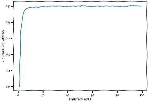
With a bit of code we can simulate thousands of death rolls and see our winrate.
We can also simulate the winrate of our opponent:
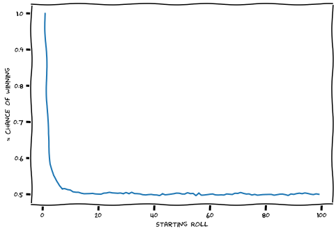
Our winrate for very small starting rolls \((2,3,4,5)\) is quite low, but nevertheless very quickly approaches a near \(50\%\) winrate as the initial roll increases.
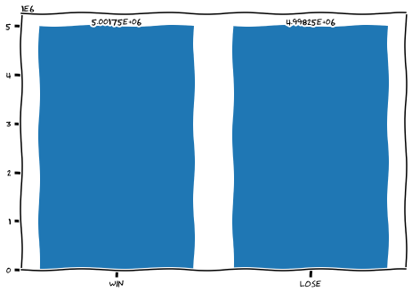
For example, if we perform \(10,000,000\) simulations with a starting roll of \(10,000\) the winrate is essentially \(50\%\).
It seems for small rolls my initial assumption was correct; however, for larger initial rolls neither side has an advantage.
Analysis
Now, we’ll try to calculate our exact chances of winning.
Let
\(g(n) = \text{expected chance of winning over losing}, -1 <= g(n) <= 1\).
So if \(g(n) = 1\) we would expect to always win, while \(g(n) = -1\) would mean we always expect to lose and \(g(n) = 0\) means we expect to lose as often as we win.
Next, we’ll draw a probability tree for a game with a starting roll of \(3\).
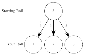
On the first roll we instantly lose \(\frac{1}{3}rd\) of the time, for roll \(2\) a \(\frac{1}{3}rd\) of the time and for roll \(3\) a \(\frac{1}{3}rd\) of the time. In the cases we roll a \(2\) or \(3\) we can draw out what the opponent’s probabilities are.
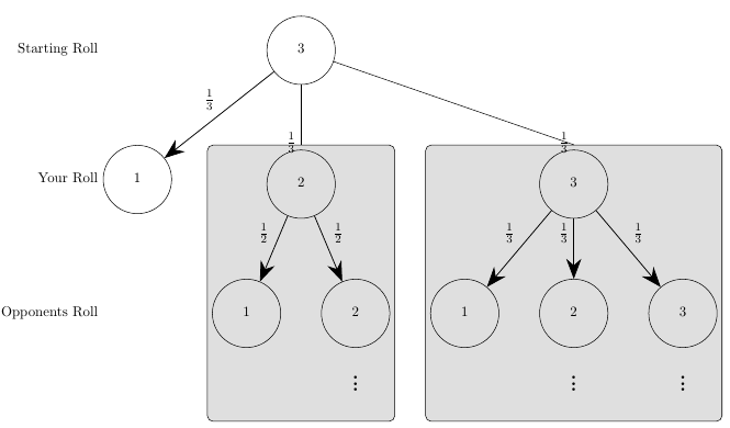
Quite quickly we see the recursive nature of this game.
Expected value is typically calculated as
\[\text{EV} = \sum{(P(X_i) \times X_i)}\]Where \(P(X_i)\) is the probability that outcome \(X_i\) occurs. In our case we have 3 outcomes: either we roll a \(\{1,2,3\}\), each having an equal probability \(P(1) = P(2) = P(3) = \frac{1}{3}\).
Therefore1
\[\begin{align} g(3) &= \frac{1}{3} \times (-1) - \frac{1}{3} \times g(2) - \frac{1}{3} \times g(3) \\ & = - \frac{1}{3} - \frac{1}{3}g(2) - \frac{1}{3}g(3) \end{align}\]Now, we need to figure out what \(g(2)\) is equal to.
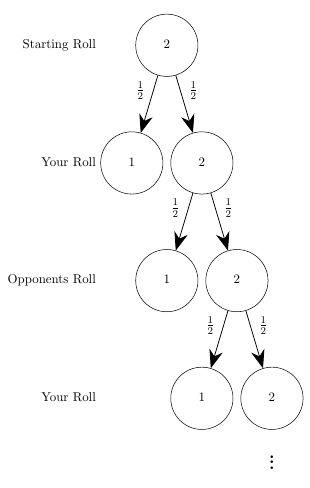
We’ll start off again by drawing its probability tree
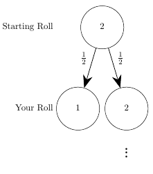
We’ll expand that several times and see if we can see any pattern.
We can apply the following identity to our above summation: \(\sum_{n=1}^{\infty}(ar^k) = \frac{ar}{1-r}, \text{iff } \vert r \vert < 1\).
\[g(2) = \frac{1 \times \frac{-1}{2}}{1 - \frac{-1}{2}} = -\frac{1}{3}\]Therefore we can expect to lose \(33.\bar{3}\%\) more games than we win. Another way to write the equation is \(g(n) = \text{win %} - \text{lose %}\). Additionally we know \(\text{win %} + \text{lose %} = 1\). Using these two equations we can express our winrate directly.
\[\begin{align} g(n) &= W(n) - L(n) \tag{1} \\ 1 &= W(n) + L(n) \tag{2} \\ &\text{Add (1) to (2)} \\ g(n) + 1 &= 2W(n) \\ \frac{g(n) + 1}{2} &= W(n) \\ \end{align}\]Using our previously calculated results
\[g(2) = - \frac{1}{3} \longrightarrow W = \frac{g(2) + 1}{2} = \frac{ -\frac{1}{3} + 1}{2} = \frac{1}{3}, L = \frac{2}{3}\]Hence, we can expect to win once every \(3\) games assuming we roll first and begin the rolls at \(2\).
Now that we’ve calculated \(g(2),\) let’s go back to \(g(3)\). From above we have
\[\begin{align} g(3) &= -\frac{1}{3} - \frac{1}{3}g(2) - \frac{1}{3}g(3) \tag{1} \\ g(2) &= -\frac{1}{3} \tag{2} \\ &\text{Substitute (2) into (1)} \\ g(3) &= -\frac{1}{3} - \frac{1}{3}(- \frac{1}{3}) - \frac{1}{3}g(3) \\ &= -\frac{1}{3} + \frac{1}{9} - \frac{1}{3}g(3) \\ &= -\frac{2}{9} - \frac{1}{3}g(3) \\ &= -\frac{2}{9} - \frac{1}{3}(-\frac{2}{9} - \frac{1}{3}g(3)) \\ &= -\frac{2}{9} +\frac{2}{27} + \frac{1}{9}g(3) \\ &= -\frac{2}{9} +\frac{2}{27} + \frac{1}{9}(-\frac{2}{9} - \frac{1}{3}g(3)) \\ &= -\frac{2}{9} +\frac{2}{27} -\frac{2}{81} - \frac{1}{27}g(3) \\ &\cdots \\ &=\sum_{n=0}^{\infty}-2\left(\frac{-1}{3}\right)^{\left(n+2\right)} \\ &=-\frac{1}{6} \end{align}\]If we continue this process we’ll see that
\[\begin{align} g(4) &= -\frac{1}{10} \\ g(5) &= -\frac{2}{30} \\ g(6) &= -\frac{1}{21} \\ \end{align}\]While these equations are helpful there doesn’t seem to be any obvious pattern that we can exploit, so instead we’ll obtain a explicit formula for \(g(n)\) through solving its recurrence equation.
Explicit Formula
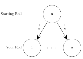
First, we’ll define \(g(n)\) recursively as
Next, we’ll define \(s(n) = \sum_{i=2}^{n}{g(i)}\) then we have that \(g(n) = - \frac{1}{n}(1 + s(n))\). We can also see that \(g(n) = s(n) - s(n - 1)\) [2]. Therefore we can plug that into the above recursive formula we have for \(g(n)\).
\[\begin{align} s(n) - s(n-1) &= -\frac{1}{n}(1 + \sum_{i=2}^{n}{g(i)}) \\ s(n) - s(n-1) &= -\frac{1}{n}(1 + s(n)) \\ (n)s(n) - (n)s(n-1) &= -1 - s(n) \\ (n+1)s(n) - (n)s(n-1) &= -1 \\ \end{align}\]Let’s guess that \(s(n) = -\frac{n-1}{n+1}\) solves the above equation as well as satisfies \(s(2) = g(2) = -\frac{1}{3}\)[3]. Thus,
\[\begin{align} g(n) &= s(n) - s(n - 1) \\ &= -\frac{n-1}{n+1} + \frac{n-2}{n} \\ &= \frac{-n^2+n+(n+1)(n-2)}{(n+1)n} \\ &= \frac{-n^2+n+n^2-2n+n-2}{(n+1)n} \\ &=-\frac{2}{(n+1)n} \end{align}\]Plugging that into our \(W(n)\) formula from above we get
\[\begin{align} W(n) &= \frac{g(n) + 1}{2} \\ &= \frac{-\frac{2}{(n+1)n} + 1}{2} \\ &= \frac{1}{2} - \frac{1}{(n+1)n} \\ \end{align}\] \[\lim_{n\to\infty} W(n) = \frac{1}{2} - \frac{1}{\infty} = \frac{1}{2}\]which if we graph out looks very similar to our simulation results.
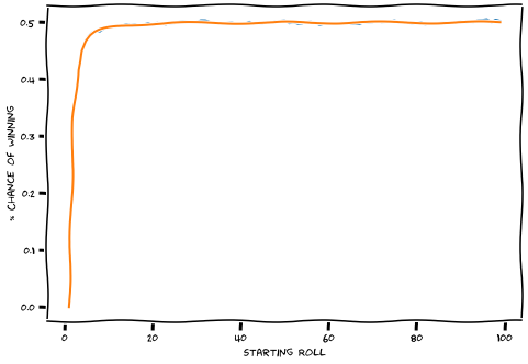
In the end we see that regardless of the starting roll the second player always has some advantage, which for sufficiently large starting rolls has negligible impact.
Death rolling, while more fun than flipping a coin, can essentially be simplified to exactly that, a \(50/50\) chance of winning or losing.
Notes
Lots of the equations/math was verified using this Desmos calculator.
[1] In the case of rolling a \(1\) we instantly lose, so we assign that a \(-1\) value and we minus the recursive cases since it’s returning the probability the opponent wins when starting to roll from \(2,3\). ↩
[2]
\(s(n) - s(n-1) = \sum_{i=2}^{n}{g(i)} - \sum_{i=2}^{n-1}{g(i)} = g(n)\).
[3]
Let’s show that \((n+1)s(n) - (n)s(n-1) = -1\) is solved by \(s(n) = -\frac{n-1}{n+1}\)
\[\begin{align} (n+1)s(n) - (n)s(n-1) &= -1 \\ -\frac{(n+1)(n-1)}{n+1} + \frac{n(n-2)}{n} &= -1 \\ -n+1+n-2 &= -1 \\ -1 &= -1 \\ \end{align}\]Big thanks to briemann from Stackexchange, he wrote most of the proof for solving the recurrence equation ↩