Introduction
In this series about image interpolation we’ll discover the inner workings of common image interpolation algorithms. Since we’ll be comparing this blog’s implementation against OpenCV certain choices were made in order to mimic OpenCV’s implementation.
Nearest Neighbour Theory
Nearest Neighbour interpolation is the simplest type of interpolation requiring very little calculations allowing it to be the quickest algorithm, but typically yields the poorest image quality.
Nearest Neighbour interpolation is also quite intuitive; the pixel we interpolate will have a value equal to the nearest known pixel value.
Let’s take a look at a simple example of going from a \(2\times2\) image to a \(4\times4\) image
| \(1\) | \(2\) |
| \(3\) | \(4\) |
We want to enlarge the above image by a factor of \(2\), ie to a \(4\times4\) image.
| \(P1\) | \(P2\) | ? | ? |
| ? | ? | ? | ? |
| ? | ? | \(P3\) | ? |
| ? | ? | ? | ? |
We’ll walk through how to calculate the value for a few specific pixels: \(P1\), \(P2\), \(P3\).
First, we need to establish our pixel coordinate system. Each pixel measures unit length and width and is defined by it’s center value coordinate. Indexing will start at \(0.5\), i.e. \(P1\) is at \((0.5, 0.5)\) and \(P2\) is at \((1.5, 0.5)\). While in the original image \(1 : (0.5, 0.5)\), \(2 : (1.5, 0.5)\), \(3 : (0.5, 1.5)\), \(4 : (1.5, 1.5)\).
| pixel value | pixel coordinate |
|---|---|
| \(1\) | \((0.5, 0.5)\) |
| \(2\) | \((1.5, 0.5)\) |
| \(3\) | \((0.5, 1.5)\) |
| \(4\) | \((1.5, 1.5)\) |
Now let’s get on with the algorithm:
- Identify the coordinates of the pixel, \(P\), we are interpolating (on the unknown image).
- Project the pixel onto the original input image. This is done by multiplying each coordinate by the scale ratio.
- Calculate the closest pixel to our projected pixel and assign \(P\) to that value.
We’ll work through the algorithm for \(P1\), \(P2\), and \(P3\).
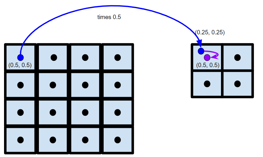
- Pixel \(P1\)
- So \(\text{P1}\) in the enlarged image has coordinates \((0.5, 0.5)\).
- Our image has a scale ratio of \(2/4\) (the scale ratio is calculated by \(\frac{\text{in\_dimension}}{\text{out\_dimension}}\)) in the x and y direction, so we’ll divide \(P1's\) x and y values by \(2\), giving us \((0.25, 0.25)\).
- Looking at our original image, \((0.25,0.25)\) is closest to \(1 : (0.5, 0.5)\). Meaning \(P1\) gets a value of \(1\).
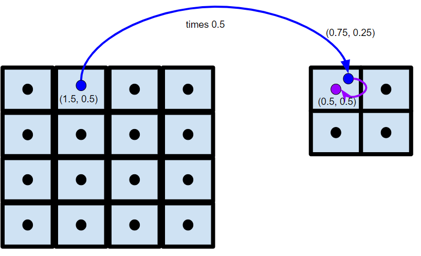
- Pixel \(P2\)
- Our pixel \(P2\) is at \((1.5, 0.5)\). When projected we’ll have coordinates \((0.75, 0.25)\), making \(1 : (0.5, 0.5)\) the closest pixel.
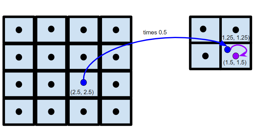
- Pixel \(P3\)
- Our pixel \(P3\) is at \((2.5, 2.5)\). When projected we’ll have coordinates \((1.25, 1.25)\), making \(4 : (1.5, 1.5)\) the closest pixel.
If we repeat this process on all the pixels in the enlarged image we end up with
| \(1\) | \(1\) | \(2\) | \(2\) |
| \(1\) | \(1\) | \(2\) | \(2\) |
| \(3\) | \(3\) | \(4\) | \(4\) |
| \(3\) | \(3\) | \(4\) | \(4\) |
Code
In this section we’ll utilize a \(0\)-index based coordinate system while keeping unit length and unit width. We utilize \(0\)-indexing to simplify the code.
Let’s write a little python code to automate this interpolation process for us. In order to mimic OpenCV we will need to utilize the same process as they do in identifying the nearest pixel. Finding the nearest pixel can be thought of as rounding i.e. a pixel at \((0.6, 0)\) has it’s nearest neighbor (by distance) at \((1, 0)\) or \(\text{def nearestPixel(x, y)} \rightarrow (\lfloor x \rceil, \lfloor y \rceil)\). Unfortunately, rounding has many definitions; here are the 5 as defined by IEEE-754.
| mode | \(11.5\) | \(12.5\) | \(-11.5\) | \(-12.5\) |
|---|---|---|---|---|
| to nearest, ties to even | \(12.0\) | \(12.0\) | \(-12.0\) | \(-12.0\) |
| to nearest, ties away from zero | \(12.0\) | \(13.0\) | \(-12.0\) | \(-13.0\) |
| toward \(0\) | \(11.0\) | \(12.0\) | \(-11.0\) | \(-12.0\) |
| toward \(+\infty\) | \(12.0\) | \(13.0\) | \(-11.0\) | \(-12.0\) |
| towards \(-\infty\) | \(11.0\) | \(12.0\) | \(-12.0\) | \(-13.0\) |
OpenCV utilizes the 3rd definition of rounding toward \(\textbf{0}\), i.e. truncating/flooring the pixel values is used to find the nearest neighbor. It’s of course perfectly valid to use other rounding rules, but it will lead to minor differences in results. This paper examines the efficiency of the various methods and provides a visual example of the consequences of different rounding rules:
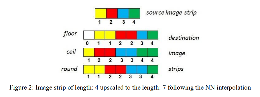
The key takeaway from this image is that regardless of the rule chosen the overall resulting images are relativity the same, except around boundary pixels, due to different precision in the rounding rules.
This github thread does a great job visually showing the potential downsides of OpenCV’s rounding rule choice. Imagine you are shrinking a \(5\times5\) image down to \(1\times1\). Typically, one would imagine you take the center pixel from the \(5\times5\) image, but due to flooring OpenCV will take the top left pixel instead. You can read more about this here. Overall Nearest Neighbour interpolation trades image quality for efficiency, as a result minor inconsistencies between implementations can be expected.
Now let’s get to the code:
import cv2
import math
import numpy as np


def nearest(input, output, sx, sy):
  for y in range(len(output)):
    for x in range(len(output[y])):
      proj_x = math.floor(x * sx)
      proj_y = math.floor(y * sy)
      output[y][x] = input[proj_y][proj_x]

a = np.array( [ 1, 2, 3, 4] ).reshape( ( 2, 2 ) )
output = np.zeros( (4, 4) )
nearest(a, output, 0.5, 0.5)
print(output)

print(cv2.resize( a.astype('float'), ( 4, 4 ), interpolation = cv2.INTER_NEAREST ))
It’s relativity simple:
- you loop over all the output pixels
- project each pixel back to the input image
- floor the projected pixel to find the nearest pixel
- assign the output pixel to the nearest pixel found
We can use the following code to do a “proof” by exhaustion by comparing our implementation’s results against OpenCV’s results.
while True:
  in_x = np.random.randint(2, 10)
  in_y = np.random.randint(2, 10)

  out_x = np.random.randint(2, 10)
  out_y = np.random.randint(2, 10)

  test = np.random.random( (in_y , in_x) )

  expected = cv2.resize(test, (out_x, out_y), interpolation = cv2.INTER_NEAREST)

  actual = np.zeros( (out_y, out_x) )
  nearest(test, actual, in_x / out_x, in_y / out_y )

  print(expected)
  print(actual)

  if not np.array_equal(actual, expected):
    print("error in code!")
    break