Calculator
Number of rows
Number of columns
Quantifying Randomness: Entropy, Information Gain and Decision Trees
Entropy
Entropy is a measure of expected “surprise”. Essentially how uncertain are we of the value drawn from some distribution. The higher the entropy the more unpredictable the outcome is. For example if I asked you to predict the outcome of a regular fair coin, you have a \(50\%\) chance of being correct. If instead I used a coin for which both sides were tails you could predict the outcome correctly \(100\%\) of the time.
Entropy helps us quantify how uncertain we are of an outcome. And it can be defined as follows1:
\[H(X) = -\sum_{x \in X}{p(x)\log_2p(x)}\]Where the units are bits (based on the formula using log base \(2\)). The intuition is entropy is equal to the number of bits you need to communicate the outcome of a certain draw.
A fair coin has \(1\) bit of entropy which makes sense as a coin can be either heads or tails, so a total of 2 possibilities which \(1\) bit can represent. A fair die’s entropy is equal to \(\simeq 2.58\). We need to represent rolls \(1-6\) which account for \(6\) possibilities. \(6\) states can be represented in binary by the following \([ 000, 001, 010, 011, 100, 101]\), so in total we need \(3\) bits, but not the entire \(3\) bits as we don’t utilize \(111\) or \(110\). Therefore it makes sense the entropy, \(H\), is between \(2\) and \(3\).2
Conditional Entropy
How does entropy change when we know something about the outcome? Lets suppose we know a day is cloudy \(49\%\) of the time, and the remaining \(51\%\) of the time it is not cloudy. The entropy of such a distribution is \(\simeq1\). Now imagine we are told if it is raining or not, with the following probabilities:
| cloudy | not cloudy | |
|---|---|---|
| raining | 24/100 | 1/100 |
| not raining | 25/100 | 50/100 |
Now what is the entropy if we know today is raining. If it is raining then it is cloudy \(24\%\) of the time and not cloudy \(1\%\) of the time. Therefore
\[H(Y \vert X = \text{raining}) = -p(\text{cloudy}\vert\text{raining})\log_2p(\text{cloudy}\vert\text{raining}) -p(\text{not cloudy}\vert\text{raining}) \\ \log_2p(\text{not cloudy}\vert\text{raining}) = -\frac{24}{25}\log_2\frac{24}{25} - \frac{1}{25}\log_2\frac{1}{25} \simeq 0.24\]\(1\) and \(0.24\) are quite different and from the table it is clear that knowing if the day is raining is very beneficial for guessing if today is cloudy.
More generically we can define specific conditional entropy as
\[H(Y \vert X) = \sum_{x \in X}p(x)H(Y \vert X = x)\] \[= -\sum_{x \in X}\sum_{y \in Y}p(x, y)\log_2p(y \vert x)\]Where
\[p(x,y) = p(x) \times p(y \vert x)\]Information Gain
This loss of randomness or gain in confidence in an outcome is called information gain. How much information do we gain about an outcome \(Y\) when we learn \(X\) is true. More formally
\[IG(Y \vert X) = H(Y) - H(Y \vert X)\]In our cloudy day scenario we gained \(1 - 0.24 = 0.76\) bits of information. If \(X\) is uninformative or not helpful in predicting \(Y\) then \(IG(Y \vert X) = 0\).
Decision Trees
What does all this talk about entropy and information gain give us? It lets us empirically define what questions we ask to have the best opportunity to predict an outcome from some distribution.
Let’s say we have the following data3:
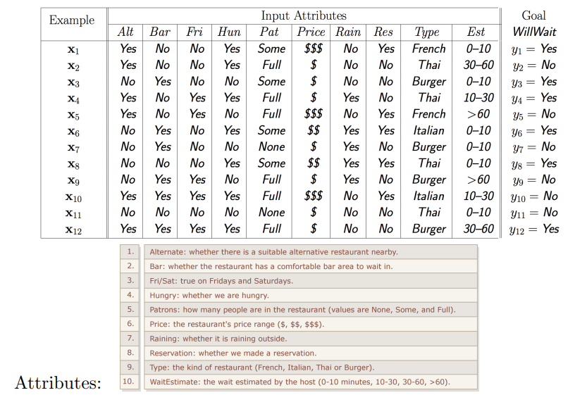
and we have another example \(x_{13}\). We want to know whether or not the customer will wait. We will use decision trees to find out!
Decision trees make predictions by recursively splitting on different attributes according to a tree structure.
An example decision tree looks as follows:
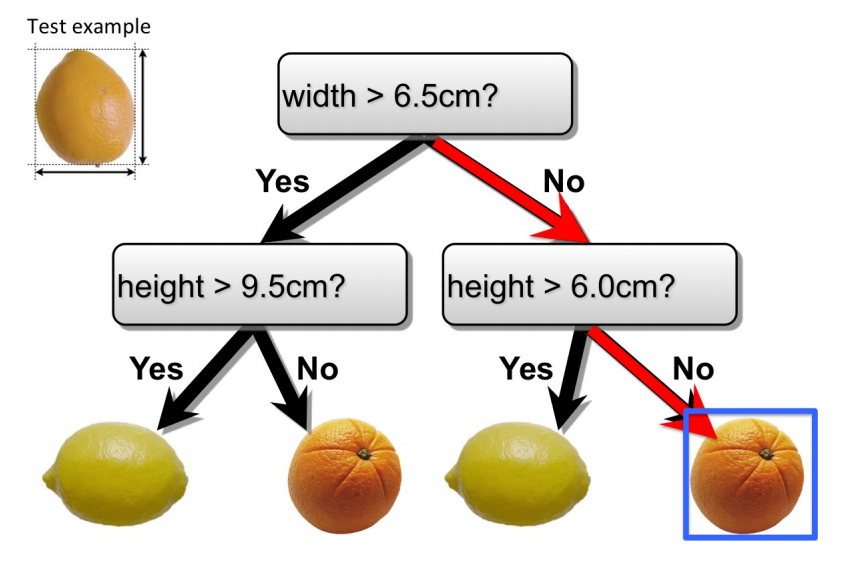
If we had an observation that we wanted to classify \(\{ \text{width} = 6, \text{height} = 5\}\), we start the the top of the tree. Since the width of the example is less than 6.5 we proceed to the right subtree, where we examine the sample’s height. Since \(5 \leq 6\) we again traverse down the right edge, ending up at a leaf resulting in a No classification.
How do we decide which tests to do and in what order? We use information gain, and do splits on the most informative attribute (the attribute that gives us the highest information gain).
In our restaurant example, the type attribute gives us an entropy of \(0\)
\[IG(Y | \text{type} ) = H(Y) - [P(\text{French})H(Y | \text{French}) + P(\text{Italian})H(Y \vert \text{Italian}) \\ + P(\text{Thai})H(Y \vert \text{Thai}) + P(\text{Burger})H(Y \vert \text{Burger})] = 0\]Therefore type is a bad attribute to split on, it gives us no information about whether or not the customer will stay or leave.
Patrons on the other hand is a much better attribute, \(IG(Y \vert \text{Patrons}) = \\ H(Y) - [P(\text{none})H(Y \vert \text{none}) + P(\text{some})H(Y \vert \text{some}) + P(\text{full})H(Y \vert \text{full})] \simeq 0.54\)
Therefore splitting on Patrons would be a good first test.
This process can continue where we pick the best attribute to test on until all discussions lead to nodes containing observations with the same label. Alternatively we can stop at some maximum depth or perform post pruning to avoid overfitting.
Now if our final decision tree looks as follows
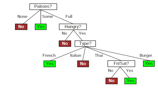
We can now predict whether \(x_{13}\) will wait or not. Lets suppose \(x_{13}\) has the following key attributes \(\{ Patrons = Full, Hungry = Yes, Type = Burger \}\). We can follow the tests in the tree to predict that \(x_{13}\) will wait.
Footnotes
[1] An interesting side-note is the similarity between entropy and expected value.
\[E(X) = \sum_{x \in X}p(x)\times x\] \[H(X) = -\sum_{x \in X}{p(x)\times\log_2p(x)}\]The two formulas highly resemble one another, the primary difference between the two is \(x\) vs \(\log_2p(x)\). We can redefine entropy as the expected number of bits one needs to communicate any result from a distribution. ↩
[2] This type of rational does not always work (think of a scenario with hundreds of outcomes all dominated by one occurring \(99.999\%\) of the time). But will serve as a decent guideline for guessing what the entropy should be. ↩
[3] Images taken from https://erdogdu.github.io/csc311_f19/lectures/lec02/lec02.pdf ↩