Introduction
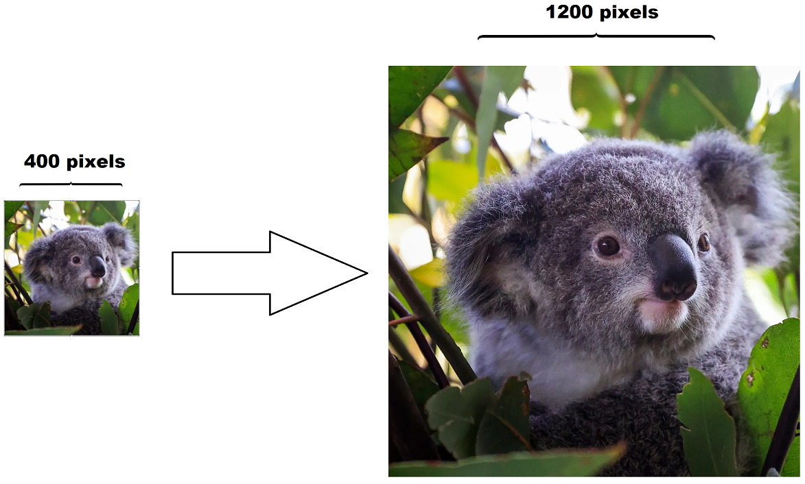
Have you ever wondered how an image can have its size doubled yet keep its original image quality? This is thanks to a technique called image interpolation which has been developed by mathematicians and researchers over hundreds of years. Some of the more intricate image interpolation formulas include: Lanczos resampling and bicubic interpolation.
Before understanding how image interpolation works, we need to better understand what an image is actually composed of. We can imagine an image as 1 or more 2d matrices where each matrix represents a channel; the most common channels are Red, Green, Blue and Alpha (commonly abbreviated to rgba). A pixel at position \((i, j)\) is represented by a tuple created by concatenating the values from each channel at \((i, j)\). For example, a pixel in a rgba image could be generally represented as \(P_{i,j} = ( R_{i,j}, G_{i,j}, B_{i,j}, A_{i,j} )\) where \(R, G, B, A\) are all matrices.

When we are resizing an image, we recreate all the channel matrices except with a different number of rows and/or columns. But what values do we put inside these new matrices? The exact process depends on the image interpolation algorithm you choose; in general, there are 2 steps which are repeated for every element in every channel. First, each element is projected onto the old matrix then using the elements surrounding the projected position we can interpolate the new elements value.
Using the graphical tool below you can dive deeper into the various interpolation techniques and learn exactly how they operate. Alternatively, visit the blog posts linked below for a deeper dive into each interpolation technique.
Simulator explanation
The simulator below is a fully interactive image interpolator. You can zoom in/out (by scrolling the mouse wheel), pan around, and edit the input image values (this can by done by double clicking the text fields on the input image).
Click on the pixels on the right-hand side to see exactly how their values were calculated.
You may notice grey squares on the input image side; these are artificially added to the image to support your chosen interpolation algorithm. These additional elements are created by copying the border elements of the input image, thus they themselves cannot be directly changed (but if the border elements are changed then the artificially added elements will update accordingly).
The pixels have unit width and length, and their position is described by the center of the pixel. For example, the top left pixel is at \((0.5, 0.5)\). This isn’t too critical to understand until you take a deeper look into the implementation of these interpolation algorithms.
To learn more about the actual math and implementation of these various interpolation methods see the blog posts below: